
If you wanted to measure the speed of a car, cheetah, or baseball, how would you go about it?
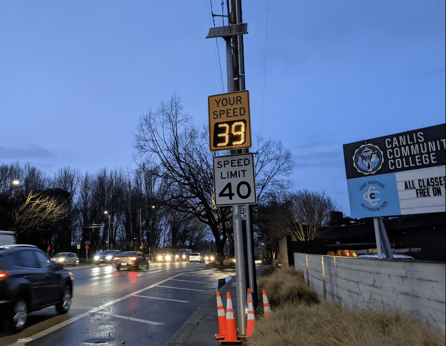
A sign that tells you your speed. (Image: sdotblog.seattle.gov)
For an object with constant speed, you might have learned the velocity formula:
\[v = \frac{\Delta x}{\Delta t}\]
To compute constant speed, we take the distance traveled and divide it by the amount of time it took to travel that distance. For example, if we see a car at mile marker \(51\) at 3:00 and then see it at mile marker \(193\) at 5:00, then \(193-51 = 142\) miles were driven in \(5-3 = 2\) hours. If the car was traveling with constant speed, then that speed was
\[ v = \frac{142 \textrm{ miles}}{2 \textrm{ hours}} = 71 \textrm{ mph} \]
For an object whose speed isn’t constant, then the same formula still works, but it gives us the object’s average velocity over that time period.
If the speed limit on the highway in our example were \(60 \textrm{ mph}\), did the car break the speed limit? Its average velocity was \(71 \textrm{ mph}\), so it seems like it would have had to be traveling faster than \(60 \textrm{ mph}\) at some point — right? That feels too obvious to be false, but how do we know that it’s true?
The mean value theorem
Calculus provides a really nice answer, which I’ll re-variable a little to suit our situation:
Mean value theorem
Let \(x(t)\) be a function continuous on a closed interval \([a,b]\) and differentiable on the open interval \((a,b)\). Then there is at least one number \(c\) in \((a,b)\) such that the instantaneous rate of change equals the average rate of change:
\[ x’(c) = \frac{x(b)-x(a)}{b-a}\]
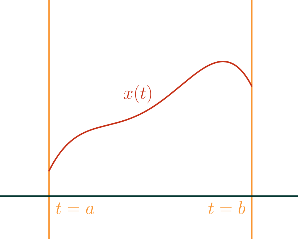
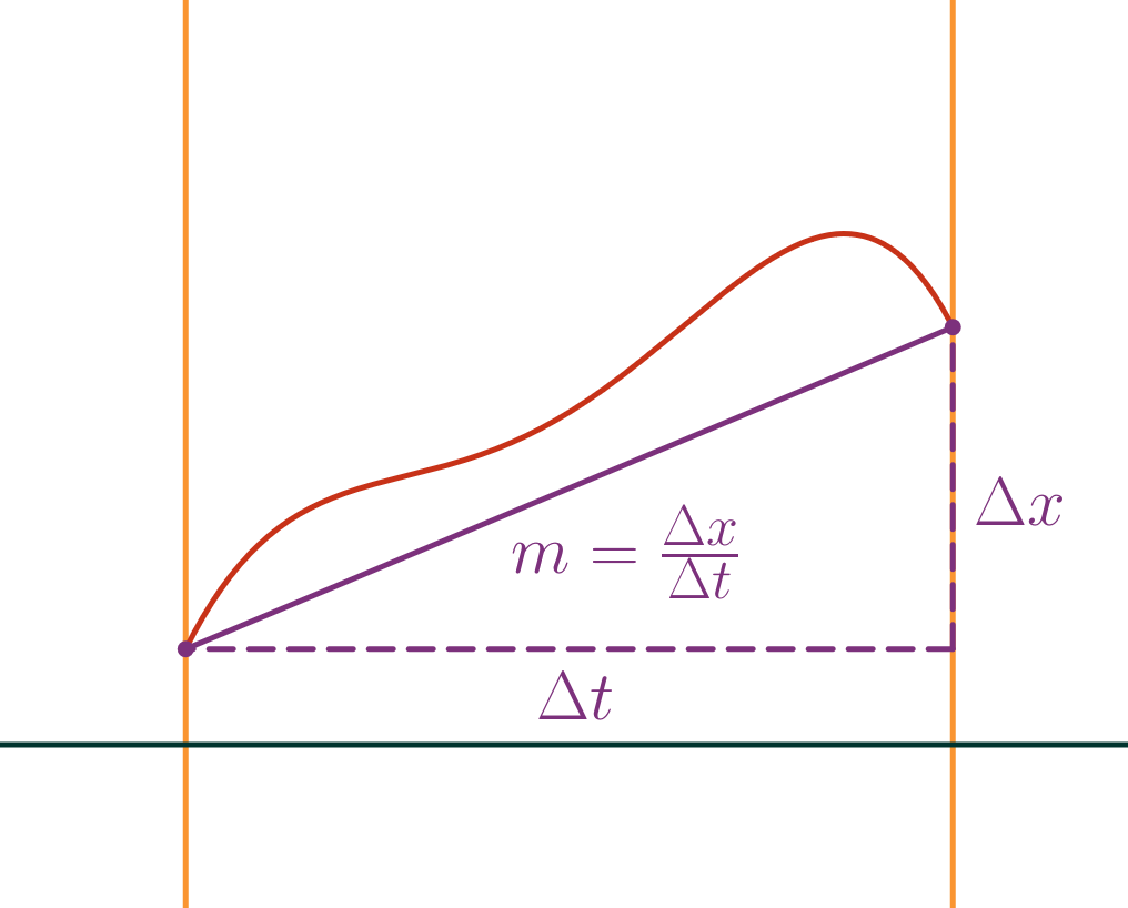
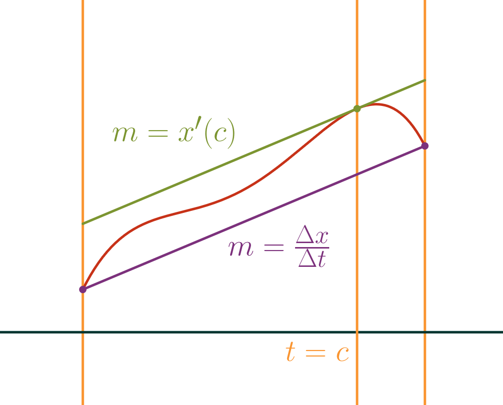
That’s all a little jargon-y, but if \(x\) is the position of an object, then its instantaneous rate of change (derivative) is what we call velocity, \({v = x’}\). Since motion for cars is smooth (continuous, differentiable, and so much more!) and since the car in our example’s average velocity was \(\frac{\Delta x}{\Delta t} = 71 \textrm{ mph}\), the mean value theorem allows us to say that there was at least one point in time \(c\) between 3:00 and 5:00 that the car’s speed was \(x’(c) = 71 \textrm{ mph}\).
If you were a highway patrol officer parked on the side of the highway and wanted to check whether a car was speeding, then one way to go about it is to check the time as it whizzes by your parked car, radio your partner, and have them check the time when it whizzes by their parked car.
If you and your partner know the distance between your cars and have synchronized watches, then you can find the average velocity of the car in the time it took driving in between. If that average is higher than the speed limit, then the car must have been speeding at some point by the mean value theorem.
On the other hand, if that average speed isn’t higher than the speed limit, then maybe the car slowed down for long enough that the time it spent driving below the speed limit effectively canceled out the time it spent driving above the speed limit in the average. So checking the average can give false negatives, but not false positives.
This method is used in the UK, Austria, Italy, and other countries, typically using cameras at the two locations instead of squad cars to recognize the speeder at both locations and log the times it was spotted. This system of clocking a vehicle at two points with known distance apart isn’t as common here in the US, where we typically measure speed by radar. When you pass a speed limit sign that shows you your speed to encourage you to slow down, for example, it’s using radar.
Radar
Radar speed measurements work by bouncing a radio wave off an object and then seeing how much the phase of the returning wave (its echo) changes. If a car has distance \(x\) from you and is moving away, then we can again think of its position as \(x(t)\), which will increase as time goes by. The phase advance of the echo will be given by
\[ \varphi(t) = \frac{4\pi x(t)}{\lambda} \]
when the car is at distance \(x(t)\), where \(\lambda\) is the wavelength of the radio wave. If we compare the phase of the echo at two times \(t = a\) and \(t = b\) that are very close together, we can compute the average angular frequency over that time interval:
\[ \frac{\varphi(b)-\varphi(a)}{b-a} = \frac{4\pi}{\lambda} \left(\frac{x(b)-x(a)}{b-a}\right)\]
Recognizing that bit in the parentheses as average velocity, we can solve for it:
\[ \frac{x(b)-x(a)}{b-a} = \frac{\lambda}{4\pi} \left(\frac{\varphi(b)-\varphi(a)}{b-a}\right)\]
We would still rely on the mean value theorem to conclude that the instantaneous velocity must equal this average velocity somewhere during the time interval, but the time interval is now only a few milliseconds long. A car will only move a few inches in that time span, so that average velocity might as well be the car’s instantaneous velocity.
Though a bill to change it is currently moving through the legislature, Pennsylvania non-state police have long been barred from using radar and have had to rely on clocking a vehicle at two points with known distance apart. On the other hand, a speed trap law in California prevent officers from clocking a vehicle at two points with known distance apart, but does allow for radar use. While they have to use different methods to catch speeders, officers in both states end up relying on the mean value theorem to establish speeds!
What other ways might you measure speed?

