
“How does a calculator work?”
Great question! I knew the gist of adding circuits, but there were some things specific to calculators I hadn’t known before digging into it. We’ll mostly look at how computers handle addition, since I think computers are a little simpler and addition is a nice, concrete process. We’ll then look at a way that a calculator’s approach often differs.
Converting to binary
The first step for any digital numerical computation is representing the numbers in binary. Our usual decimal system is based on powers of \(10\):
\[1, 10, 100, 1000, 10000, 100000, 1000000, 10000000, 100000000, 1000000000, 10000000000, 100000000000, …\]
Binary is similarly a place value system, but based on powers of \(2\):
\[1, 2, 4, 8, 16, 32, 64, 128, 256, 512, 1024, 2048, 4096, 8192, 16384, 32768, 65536, 131072, 262144, 524288, …\]
When I convert a number to binary, I usually go about it by finding the largest power of \(2\) not larger than my number, subtracting it, and repeating with that difference. Once I get a difference of \(0\), the powers of \(2\) I used tell me where to put the \(1\)’s in the binary representation. For example, with \(53\),
\[ {\color{#c83219} 32 } \leq 53 < 64, \qquad 53-32 = 21 \]
\[ {\color{#c83219} 16 } \leq 21 < 32, \qquad 21-16 = 5 \]
\[ {\color{#c83219} 4 } \leq 5 < 8, \qquad 5-4 = 1 \]
\[ {\color{#c83219} 1 } \leq 1 < 2, \qquad 1-1 = 0 \]
Keeping track of which powers of \(2\) we used (and which we didn’t), we can write
\[ \begin{eqnarray} 53 & = & {\color{#c83219} 32 } + {\color{#c83219} 16 } + {\color{#c83219} 4 } + {\color{#c83219} 1 } \\ && \\ & = & {\color{#c83219} 1 } \cdot {\color{#c83219} 32 } + {\color{#c83219} 1 } \cdot {\color{#c83219} 16 } + 0 \cdot 8 + {\color{#c83219} 1 } \cdot {\color{#c83219} 4 } + 0 \cdot 2 + {\color{#c83219} 1 } \cdot {\color{#c83219} 1 } \\ && \\ & = & {\color{#c83219} 11}0 {\color{#c83219} 1}0{\color{#c83219} 1}_{\color{#fa9632} 2} \end{eqnarray} \]
Try finding the binary representations of some target numbers yourself by clicking boxes corresponding to the powers of \(2\) you think should have a \(1\) in its representation. (For example, for \(53\), you’d click boxes \(64\), \(32\), \(4\), and \(1\).)
When having a program find binary representations, I’d probably code it in terms of division and remainders mod \(2\), but this should give you enough of an idea of where binary strings of \(0\)’s and \(1\)’s come from.
Binary addition
There were a few games making the rounds while I was in grad school all based on a similar idea. I think the original was Sirvo’s Threes, but the variants 1024 and 2048 caught on faster. If you’ve played it, perhaps you felt a little nostalgic while building binary numbers with the interface above! If you haven’t played it, see if you can figure out the rules to 1024 by playing with the app below. You can click the board to use your keyboard to push all tiles, up, left, down, or right or just press the arrow buttons below.
I like to think of binary addition as a simple version of 1024, where like powers of \(2\) merge in chain reactions until at most one copy of each is left. Try adding a few pairs of numbers and see if you can figure out what’s going on:
If you’ve ever done the standard addition algorithm where you line up two numbers and add the digits that are vertically stacked, possibly carrying \(1\)’s, what’s happening in binary is the same principle. We carry a \(1\) in decimal addition when the sum of two digits is larger than the greatest possible digit, \(9\). In binary, we also carry a \(1\) when the sum of two digits is larger than the greatest possible digit, which is \(1\). In the app above, you’re seeing a carry occur whenever a too-large power of \(2\) moves left one column.
Here’s what binary addition looks like longhand for \(1111_{\color{#fa9632} 2} + 1010_{\color{#fa9632} 2}\):
\[\begin{matrix} & {\tiny\color{#7d327d} 1 } & {\tiny\color{#7d327d} 1 } & {\tiny\color{#7d327d} 1 } && \\ & & 1 & 1 & 1 & 1_{\color{#fa9632} 2} \\ + & & 1 & 0 & 1 & 0_{\color{#fa9632} 2} \\ \hline & 1 & 1 & 0 & 0 & 1_{\color{#fa9632} 2} \end{matrix}\]
Logic gates
Now that we know how binary addition works in terms of place value and carries, let’s look at how computers actually do it.
The basic building blocks for making digital circuits called logic gates. Logic gates work by taking in one or more values \(0\) or \(1\) and returning a value \(0\) or \(1\). In electronics, these values have the physical forms of low voltage (\(0\)) and high voltage (\(1\)).
Three common logic gates are AND, OR, and XOR.
AND takes in two inputs, returning \(1\) if both inputs are \(1\) and returning \(0\) otherwise.
OR takes in two inputs, returning \(1\) if at least one input is \(1\) and returning \(0\) otherwise.
XOR takes in two inputs, returning \(1\) if they are different and returning \(0\) if they are the same.
Adders
No logic gate by itself is an adder, but we can use AND, OR, and XOR to build an adder. Let’s think through building an adder step by step:
When adding two binary numbers digit by digit, we can think of the stacked pair of digits as two inputs, which can only be \(0\) or \(1\). These are the output binary sums I would like to see when adding two single digits:
\[ \begin{matrix} & 0 \\ + & 0 \\ \hline & 0 \end{matrix} \qquad \begin{matrix} & 0 \\ + & 1 \\ \hline & 1 \end{matrix} \qquad \begin{matrix} & 1 \\ + & 0 \\ \hline & 1 \end{matrix} \qquad \begin{matrix} && 1 \\ + && 1 \\ \hline & 1 & 0_2 \end{matrix} \]
The main issue is that that last one returns a double-digit number. That leading \(1\) is the carry digit. If we ignore it, these sums are just an XOR. So our first step can be running our input digits through an XOR gate to get that ones digit.

If we end up with a carry digit, we’ll need to know about it for our calculation. A carry happens when both of our input digits are a \(1\), which is exactly when an AND gate returns \(1\). So we can send our input digits through an AND gate to get the carry digit.
A nice way to think about this is that, if we write all of our sums as two-digit numbers, the XOR is the ones/right digit and the AND is the twos/left digit.
\[ \begin{matrix} && 0 \\ + && 0 \\ \hline & 0 & 0_2 \end{matrix} \qquad \begin{matrix} && 0 \\ + && 1 \\ \hline & 0 & 1_2 \end{matrix} \qquad \begin{matrix} && 1 \\ + && 0 \\ \hline & 0 & 1_2 \end{matrix} \qquad \begin{matrix} && 1 \\ + && 1 \\ \hline & 1 & 0_2 \end{matrix} \]
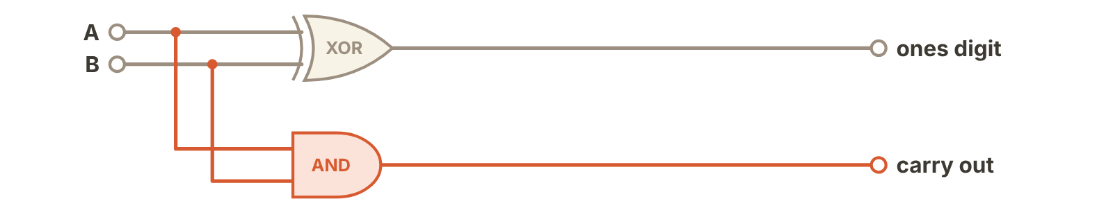
While we’re on the topic of carrying, sometimes we really need to add three digits instead of two, since there might be a carry digit from the previous sum. To distinguish between the two types of carries, we’ll call what we carry from the previous calculation a carry in while what we carry to the next calculation is carry out, as hinted in the image above.
If a carry in changes the ones digit, it’s similarly going to do it the same way an XOR would, so we can XOR our carry in digit with whatever the ones digit would have been without it.
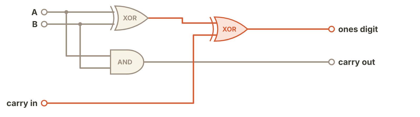
If the carry in changes whether or not there is a carry out, then it must be because our two input digits were a \(0\) and a \(1\), which is precisely when the output of our first XOR is \(1\). This means that a carry out will happen if both input digits are \(1\) OR if the that first XOR returns \(1\) AND there is a carry in. So we can augment our circuit using an AND gate and an OR gate to compute the carry out based on the carry in.
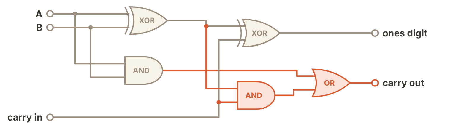
The above circuit is what’s usually called a full adder. If you were following the logic closely, you might have noticed that we could use another XOR instead of the OR, but OR gates tend to be cheaper than XORs.
To add a number with more than one digit, you can combine full adders into a ripple adder. In a ripple adder, we hook the carry out from the previous digit’s adder to the carry in on the next digit’s adder. The first carry in is fed a \(0\) and the last carry out goes to a lead digit that gets tacked on the front if a \(1\). The output ones digits together with the lead digit can be read off to get the binary sum.
Try adding some numbers with this ripple adder and watch how the signals move through it:
There are other types of adders that can use the same inputs to compute a little faster, but the idea is always to figure out a circuit of logic gates that can compute what needs to be computed. (How might you design a logic circuit that does subtraction? Multiplication? Division?)
Binary-coded decimals
If you’ve programmed, you might have noticed eccentricities in how addition works. For example, if I ask Python to compute \(0.1+0.2\), it spits out
\[ 0.30000000000000004 \]
What’s up with that?
When we express fractions as decimals, some terminate (e.g., \(1/2 = 0.5\)) and some don’t (e.g., \(2/3 = 0.\overline{6} = 0.666666…\)). If a calculator only has enough memory to store ten places past the decimal, then \(2/3\) would get truncated to become \(0.6666666666\) or rounded to become \(0.6666666667\). Entering \(2/3 + 2/3\) into a calculator would then give
\[ 0.6666666666 + 0.6666666666 = 1.3333333332 \]
or
\[ 0.6666666667 + 0.6666666667 = 1.3333333334 \]
While \(1/10 = 0.1\) terminates in decimal, as a binary number it does not: \(1/10 = 0.0\overline{0011}_2\). When Python saves \(0.1\) as a floating point number, it can’t save infinitely many digits, so it will truncate after some number of digits. Then it will decide whether it can get a little closer to the true value by rounding. Any truncation of \(0.0\overline{0011}_2\) will be smaller than \(0.1\), but adding \(1\) the the last decimal spot (and carrying, as necessary) will give a value bigger than \(0.1\). These under- and overestimates are the closest values to \(0.1\) that Python can store. Python then saves whichever of the two is actually closest to \(0.1\). In this case, it stores the overestimate.
Many calculators try to avoid this by saving things in a more decimal-friendly form of binary. Instead of saving a decimal number like \(72\) in binary as the single binary value \(1001000_2\), it will instead save each digit separately: \(0111_2 \, 0010_2\). A number stored like this is a binary-coded decimal (BCD). While this won’t make much of a difference for integers, since they don’t have repeating binary expansions (other than their infinitely many leading and trailing zeros), it can help store decimal numbers with values after the decimal point. Our addition algorithm needs to be tweaked to handle these representations along with the logic circuit to carry it out, but this stops calculators from giving the rounding “errors” that Python and many other programming languages give.

